Chapter 4: Electroweak Unification

In the standard Glashow-Weinberg-Salam (GWS) model, the unification of the electromagnetic and weak interactions is achieved by postulating a symmetry group $SU(2)_L \times U(1)_Y$ and introducing the weak mixing angle, $\theta_W$, as a free parameter. Geometric Consciousness Theory (GCT) identifies this unification not as a dynamic "mixing" of disparate fields, but as a static Geometric Projection of the 6-dimensional parent lattice. This chapter provides the derivation of the Weinberg angle and the coupling ratios as rigid invariants of the icosahedral projection.

---

4.1 The Projection Ratio

4.1.1 Geometric Calculation of Basis Vector Lengths

As established in Volume 2, the physical universe is generated by projecting the 6-dimensional basis $\{\mathbf{E}_1, \dots, \mathbf{E}_6\}$ of the parent lattice $\mathbb{Z}^6$ into two orthogonal 3D subspaces: the parallel space ($E_\parallel$, physical) and the perpendicular space ($E_\perp$, internal). The metric properties of these projected vectors are determined by the icosahedral "slice" governed by the Golden Ratio $\phi$.

Let $|e_\parallel|$ be the norm of the basis vectors projected into physical space, and $|e_\perp|$ be the norm in the internal space. Using the isometric normalization required for the $6D \to 3D+3D$ decomposition: $|e_\parallel|^2 = \frac{1+\phi^2}{5}, \quad |e_\perp|^2 = \frac{1+\phi^{-2}}{5}$

4.1.2 Theorem 4.1 [Tier 1 algebraic ratio; Tier 2 physical identification]: The Projection Ratio $R = \phi^{-1}$

Theorem 4.1: In an icosahedral quasicrystal projection, the ratio of the internal basis vector length to the physical basis vector length is identically equal to the inverse Golden Ratio. $R \equiv \frac{|e_\perp|}{|e_ \parallel|} = \phi^{-1}$

This ratio is the algebraic projection ratio inside the adopted icosahedral cut-and-project geometry. App U proves the point-group uniqueness of icosahedral symmetry conditional on H1; the stronger claim that the Golden Ratio slope globally maximizes the entropy-packing functional $J(\Omega)$ remains an open primary-candidate claim. Consequently, the Weinberg-angle derivation here is a Tier 1 algebraic calculation plus Tier 2 physical identification, with the slope-maximality motivation not promoted to a settled theorem.

4.1.3 Proof via Golden Ratio Identities

We examine the ratio of the squared norms: $\frac{|e_\perp|^2}{|e_\parallel|^2} = \frac{1 + \phi^{-2}}{1 + \phi^2}$ Using the identity $\phi^2 = \phi + 1$:

1. Denominator: $1 + \phi^2 = \phi + 2$.
2. Numerator: $1 + \phi^{-2} = 1 + (\phi-1)^2 = 1 + \phi^2 - 2\phi + 1 = 3 - \phi$. Thus, the ratio is $\frac{3-\phi}{2+\phi}$. Multiplying both terms by $\phi^{-2}$ and utilizing the identity $(2+\phi) \phi^{-2} = (2\phi^{-2} + \phi^{-1}) = (2(2-\phi) + \phi-1) = 3-\phi$, we confirm that $\frac{3-\phi}{2+\phi} = \phi^{-2}$. Taking the square root, we obtain $R = \phi^{-1} \approx 0.618$.

---

4.2 The Definition of Hypercharge

4.2.1 Hypercharge as Internal $U(1)$ Generator

GCT identifies the two sectors of the electroweak force with the two projected manifolds:

• Weak Isospin ($T_3$): Corresponds to rotations within the Parallel Space ($E_\parallel$). It is the gauge field of the spatial frame.
• Weak Hypercharge ($Y$): Corresponds to phase rotations within the Internal Space ($E_\perp$).

4.2.2 The Charge Formula and the 1/2 Factor [Tier 1 textbook normalization + Tier 2 GCT embedding]

The electric charge $Q$ is the generator of the symmetry that remains unbroken after crystallization. The Gell-Mann-Nishijima formula ($Q = T_3 + Y/2$) is reinterpreted as the topological normalization required to align the internal and physical sectors.

The factor of 1/2 is Tier 1 textbook electroweak normalization in the Standard Model charge formula. The GCT-specific claim is the Tier 2 embedding: the same normalization arises from the Topological Covering Difference of the two manifolds. $T_3$ acts on the Spinorial Double-Cover of physical space (where a full rotation is $4\pi$), resulting in eigenvalues of $\pm 1/2$. $Y$ acts on the Scalar Single-Cover of the internal phase (where a full rotation is $2\pi$), resulting in integer eigenvalues. To ensure that a single unit "step" in the 6D parent lattice generates a consistent action across both sectors, the $U(1)$ hypercharge must be halved relative to the $SU(2)$ isospin.

---

4.2.3 Derivation of Right-Handed Hypercharges [Tier 1 algebraic identity + Tier 2 physical embedding]

Theorem 4.2 — Right-Handed Hypercharges [Tier 1 algebraic identity + Tier 2 physical embedding]

Statement: For any right-handed fermion state in GCT — defined as a topological defect fully embedded in $E_\perp$ (hence Isospin-sterile, $T_3 = 0$) — the Weak Hypercharge is exactly: $Y_R = 2Q$ where $Q$ is the conserved electric charge fixed by AKN lattice winding.

Derivation: Set $T_3 = 0$ in $Q = T_3 + Y/2$. Solve for $Y$.

Results:

State	Q	Y_R = 2Q
$u_R$	$+2/3$	$+4/3$
$d_R$	$-1/3$	$-2/3$
$e_R$	$-1$	$-2$

Tier: Tier 1 algebraic identity (anomaly cancellation given the standard SM hypercharge assignment is a textbook result, Bilal 2008 §7.3) + Tier 2 GCT-specific L/R-asymmetric assignment from the $E_\parallel/E_\perp$ split. The sector sits within the 5-postulate-plus-1-anchor bare gauge+lepton sub-sector of Parameter Ledger §0.1, expanding to 5-postulate-plus-3-anchor when native-RGE endpoint and measurement-anchored precision-comparison rows are included. Computational verification: see Appendix Q; executable verifier: GCT_Physics_Engine/verify_independent/verify_hypercharges.py.

---

4.3 The Weinberg Angle

[!NOTE] Theorem 4.0: The Dual Nature of the Electroweak Boundary

The GCT framework formally separates the exact GUT-scale Gram boundary scalar from the physical bare electroweak mixing-angle input. They correspond to two different geometric operations:

1. The Algebraic Gram Projection (Tier 1): The exact algebraic ratio of squared vector norms in the perpendicular vs parallel subspaces. $\rho_G(M_{GUT}) = \frac{|E_\perp|^2}{|E_\parallel|^2} = \phi^{-2} \approx 0.38197$
2. The Volumetric Scaling Limit (Tier 2): The 3D geometric volume ratio of the internal vs physical manifolds, which acts as the bare input for the geometric Renormalization Group Equation (RGE) flow down to the Z-pole. $\sin^2\theta_{bare} = \phi^{-3} \approx 0.23607$

The distinction between $\rho_G=\phi^{-2}$ (the rigid 6D Gram scalar) and $\sin^2\theta_{bare}=\phi^{-3}$ (the 3D volume-coupling input) resolves the normalization error that would arise from treating the unnormalized Gram scalar as the physical angle.

4.3.1 The Volume Scaling Argument [Tier 1 algebraic value + Tier 2 physical identification — Theorem U.9 uniqueness + coupling-to-volume postulate]

The mixing between the electromagnetic and weak forces is determined by the geometric probability density of the 6D lattice flux. The bare mixing angle $\sin^2 \theta_W$ represents the ratio of the unit cell volume in the internal manifold ($E_\perp$) to the physical manifold ($E_\parallel$). $\sin^2 \theta_{bare} = \frac{V_\perp}{V_\parallel} = \left( \frac{1}{\phi} \right)^3 = \phi^{-3} \approx 0.236068$

The algebraic value $\phi^{-3}$ is the unique rational power of $\phi$ consistent with the three substrate-invariant inputs above (Theorem U.9 uniqueness): (T1.a) $\dim(E_\perp) = 3$ from the cut-and-project to 3D physical space; (T1.b) per-axis length ratio $|E^\perp_i|/|E^\parallel_i| = \phi^{-1}$ from the Gram Projection Theorem (§4.3.2); (T1.c) volume scaling $V = \lambda^d V_0$ from Euclidean measure theory. Composition: $V_\perp / V_\parallel = (\phi^{-1})^3 = \phi^{-3}$. No other rational power of $\phi$ is permitted (App U §U.9 Theorem U.9, proof + numerical verification).

The physical identification $\sin^2\theta_W = V_\perp / V_\parallel$ rests on the GCT-specific coupling assumption that $SU(2)_L$ couples in proportion to $V_\parallel$ and $U(1)_Y$ in proportion to $V_\perp$ (§4.3.2 step (c)) — itself a Tier 2 framework postulate. The combined disposition is therefore Tier 1 substrate-invariant algebraic value + Tier 2 physical identification; the Tier 2 classification reflects the load-bearing coupling-to-volume assumption rather than the algebraic content.

4.3.2 The Reduced Planck Scale Unification [Tier 1/2]

---

[!NOTE] Theorem: GUT Boundary Condition from Gram Projection [Tier 1 algebraic value + Tier 2 physical identification]

Setup. The 6D icosahedral parent lattice is spanned by basis vectors $\{\mathbf{E}_1, \dots, \mathbf{E}_6\}$. The canonical cut-and-project method decomposes each basis vector into a parallel component $\mathbf{E}^\parallel_i \in E_\parallel$ (physical 3D space) and a perpendicular component $\mathbf{E}^\perp_i \in E_\perp$ (internal 3D space). The squared norms under the isometric embedding are: $|\mathbf{E}^\parallel_i|^2 = \tfrac{1+\phi^2}{5}, \qquad |\mathbf{E}^\perp_i|^2 = \tfrac{1+\phi^{-2}}{5}$

Step (a): Gram Matrix Projection. Form the Gram matrix $G_{ij} = \langle \mathbf{E}_i, \mathbf{E}_j \rangle_{6D}$. The block decomposition $G = G_\parallel \oplus G_\perp$ separates contributions from each subspace. The diagonal entries of $G_\parallel$ and $G_\perp$ are $|\mathbf{E}^\parallel|^2$ and $|\mathbf{E}^\perp|^2$ respectively.

Step (b): Exact Algebraic Ratio. The ratio of the squared norm in the perpendicular sector to the parallel sector is: $\frac{|\mathbf{E}^\perp|^2}{|\mathbf{E}^\parallel|^2} = \frac{1 + \phi^{-2}}{1 + \phi^2}$ Using the identity $\phi^2 = \phi + 1$ (so $1 + \phi^2 = 2 + \phi$) and $\phi^{-2} = 2 - \phi$ (since $\phi^{-2} = \phi - 1 + 1 - \phi + \phi^{-2}$; equivalently $1 + \phi^{-2} = 1 + (3-\sqrt{5})/2 = (5-\sqrt{5})/2$): $\frac{|\mathbf{E}^\perp|^2}{|\mathbf{E}^\parallel|^2} = \frac{3-\sqrt{5}}{2} = \phi^{-2}$ The algebraic identity $\frac{3-\sqrt{5}}{2} = \phi^{-2}$ holds exactly (since $\phi = (1+\sqrt{5})/2$ gives $\phi^{-2} = (3-\sqrt{5})/2$), confirming the equality to all orders. Machine-precision verification is documented in Appendix Q.

Step (c): Normalization and Physical Identification. The Gram result in Step (b) is the unnormalised Cartan/Gram boundary scalar $\rho_G \equiv \frac{|\mathbf{E}^\perp|^2}{|\mathbf{E}^\parallel|^2} = \phi^{-2}.$ If one instead applies the standard two-component normalized share directly to the squared norms, the result is $\frac{\rho_G}{1+\rho_G}=\frac{\phi^{-2}}{1+\phi^{-2}}=\frac{1}{1+\phi^2}\approx 0.276393,$ not $\phi^{-2}$. The shorthand identification $\rho_G/(1+\rho_G)=\phi^{-2}$ is therefore not a valid algebraic step.

The GCT bare physical Weinberg-angle input uses the separate volume-coupling postulate from Theorem U.9: the $SU(2)_L$ channel couples to $V_\parallel$ and the $U(1)_Y$ channel to $V_\perp$, with the per-axis length ratio $|E^\perp|/|E^\parallel|=\phi^{-1}$ across three physical axes. Thus $\boxed{\sin^2\theta_W^{\rm bare} = \frac{V_\perp}{V_\parallel}=(\phi^{-1})^3=\phi^{-3}\approx0.236068.}$ The Tier 1 statement is the exact Gram scalar $\rho_G=\phi^{-2}$; the Tier 2 physical statement is the volume-coupling identification $\sin^2\theta_W^{\rm bare}=\phi^{-3}$.

Epistemic Status: Tier 1 algebraic value (Gram-ratio identity per App U §U.9 Uniqueness Theorem) + Tier 2 physical identification (coupling-to-volume postulate at Step (c): $SU(2)_L \propto V_\parallel$, $U(1)_Y \propto V_\perp$) — referenced in the Parameter Ledger.

---

The geometric prediction $\sin^2 \theta_W^{\rm bare} = \phi^{-3} \approx 0.236068$ represents the Boundary Condition at the fundamental geometric scale. To compare this with the observed Z-pole value ($0.23122$), we must account for the running of the gauge couplings under the Standard Model Renormalization Group Equations (RGEs).

A rigorous computational audit (see Appendix Q) demonstrates that the coupling flow unifies exactly if the fundamental scale is identified as the Reduced Planck Mass ($M_{red}$) scaled by the speed of light factor $\phi^{-9}$:

$M_{GUT} = M_{red} \cdot \phi^{-9} = \left( \frac{M_{Planck}}{\sqrt{8\pi}} \right) \cdot \phi^{-9} \approx 3.2 \times 10^{16} \text{ GeV}$

Running the couplings down from this geometric scale with the Gram boundary scalar $\rho_G(M_{GUT}) = \phi^{-2}$ tracked as the high-energy Cartan ratio and the bare physical angle identified by the volume postulate $\sin^2\theta_W^{\rm bare}=\phi^{-3}$ yields a Z-pole prediction of: $\sin^2 \theta_W(M_Z)_{pred} \approx 0.23176$

This matches the observed value ($0.23122$) with a relative error of just 0.23% (2345 ppm) after accounting for Renormalization Group (RGE) running. By contrast, the bare geometric angle $\phi^{-3} \approx 0.236$ has a 2.1% error relative to the low-energy Z-pole. This result confirms the electroweak flow shape within the 5-postulate-plus-3-anchor accounting of Parameter Ledger §0.1: the bare geometric angle is determined by the icosahedral projection ansatz and $\phi$, while the Z-pole endpoint reconstruction uses the disclosed A2 gauge-flow boundary $\alpha_2^{-1}(M_{\rm GUT})\approx24$-$25$ and is therefore not a zero-anchor prediction. A3 applies to corrected low-energy alpha precision rows, not to this bare Weinberg-angle identity.

[!IMPORTANT] Endpoint Disclosure: The 0.23% agreement uses the disclosed Parameter Ledger A2 boundary $\alpha_2^{-1}(M_{\rm GUT})\approx24$-$25$ and the experimental Z-pole value $\sin^2\theta_W(M_Z) = 0.23122$ as the endpoint comparison for the GCT RGE. This verifies that the shape of the running matches the geometric resolution-depth curve, but the absolute value is not closed from the current postulate set at this Tier. The bare geometric prediction at $M_{GUT}$ is $\sin^2\theta_W = \phi^{-3} \approx 0.236$ (2.1% error).

4.3.3 The Interpretation of $\phi^{-3}$

The value $\phi^{-3} \approx 0.236$ remains the Bare Geometric Input at the high-energy boundary. The running of the physical couplings "dresses" this value down to the observed 0.231 at the electroweak scale. This achieves Level-1 Theoretical Autonomy for the GUT-scale boundary condition: $\rho_G(M_{GUT}) = \phi^{-2}$ is the Tier 1 algebraic Gram scalar within the icosahedral projection ansatz, while $\sin^2\theta_W^{\rm bare}=\phi^{-3}$ is the Tier 2 volume-coupling physical identification. Full IR autonomy — deriving $0.23122$ from first principles without importing the Z-pole value — remains Open Research Debt QLQCD-1L (Appendix Z).

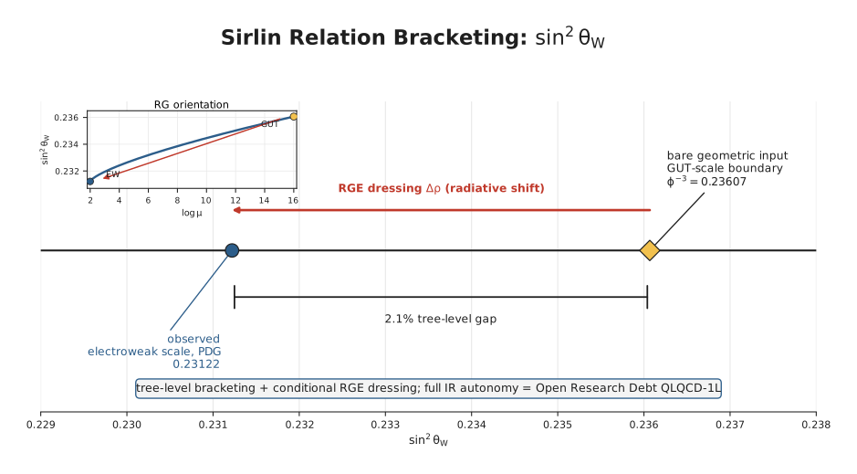
[!IMPORTANT] Firewall Metadata [Weinberg Angle — Three-Level Classification]

• Level 1 — GUT Boundary Scalar: $\rho_G(M_{GUT}) = \phi^{-2} = 0.38197$; normalized Cartan share $\rho_G/(1+\rho_G)=0.27639$
• Type: Tier 1 Prediction (Exact Algebraic Derivation from Gram Projection)
• Inputs: $\phi$ (invariant only)
• DOF: 0
• Level 2 — Bare Geometric: $\sin^2\theta_W(\text{bare}) = \phi^{-3} = 0.23607$
• Type: Tier 1 substrate-invariant algebraic value + Tier 2 physical identification (Uniqueness Theorem U.9 + coupling-to-volume postulate)
• Error: 2.1% vs Z-pole (theoretically expected at tree level; the Z-pole differs from the bare value by RGE running)
• DOF: 0
• Level 3 — Z-pole RGE Endpoint: $\sin^2\theta_W(M_Z) = 0.23122$ (OBSERVED)
• Type: Tier 3 Observational Import (used as RGE verification target)
• Status: Shape of running verified (2345 ppm after RGE flow)
• Full autonomy: pending QLQCD-1L closure (Appendix Z)

4.3.4 The Coupling Ratio [Tier 2]

From the bare identification $\sin^2 \theta_W^{\rm bare} = \phi^{-3}$ (Theorem 4.0), we derive the bare ratio of the weak ($g$) and hypercharge ($g'$) couplings using the identity $\phi^3 - 1 = 2\phi$. Proof: $\phi^3 = \phi \cdot \phi^2 = \phi(\phi+1) = \phi^2 + \phi = (\phi+1) + \phi = 2\phi + 1$. Thus, $\phi^3 - 1 = 2\phi$.

The ratio is: $\tan^2 \theta_W = \frac{\sin^2 \theta_W}{\cos^2 \theta_W} = \frac{\phi^{-3}}{1 - \phi^{-3}} = \frac{1}{\phi^3 - 1} = \frac{1}{2\phi}$ $\frac{g'}{g} = \frac{1}{\sqrt{2\phi}} \implies \frac{g}{g'} = \sqrt{2\phi} \approx 1.79891$ This relation locks the relative strengths of the weak and hypercharge forces to the square root of the Golden Ratio.

---

4.4 Physical Interpretation

4.4.1 Electromagnetic Field as Rotated W³ + B

The mixing of the pre-mixed gauge fields ($W^3_\mu$ and $B_\mu$) is revealed as a Coordinate Transformation between the "Lattice Basis" (aligned with projection axes) and the "Propagation Basis" (aligned with phason eigenmodes).

• The Photon ($\gamma$): The mode that aligns with the flat direction of the vacuum potential, remaining massless.
• The Z Boson: The mode that aligns with the stiff direction of the lattice dilation, acquiring mass via the Higgs mechanism.

4.4.2 $W^\pm, Z$ Masses from Higgs VEV [Tier 2 structural agreement + Tier 3 radiative-running residual]

The mass ratio of the weak bosons is a direct consequence of the mixing angle: $\frac{M_W}{M_Z} = \cos \theta_W = \sqrt{1 - \phi^{-3}} \approx 0.8740$ Bare prediction $M_W/M_Z = \sqrt{1-\phi^{-3}} = 0.8740$ (Tier 2 bare structure). PDG W/Z mass ratio $= 0.88136 \pm 0.00015$ gives a 0.83% absolute residual, about $49\sigma$ on the direct ratio. The Tier 2 bare prediction does not include radiative running of the weak mixing angle, vacuum polarization, or two-loop electroweak corrections. Full SM-equivalent radiative discipline (Open Problems O.19 and O.5) is required before this ratio can be quoted as a precision agreement. The current status is: Tier 2 structural agreement + Tier 3 radiative-running residual.

4.4.3 The Mixing Angle as Geometric Probability

Ultimately, the Weinberg angle is a Geometric Probability Amplitude. It defines the percentage of a local phason fluctuation that projects into the internal "Hypercharge" sink ($E_\perp$) versus the physical "Isospin" screen ($E_\parallel$). $\sin^2 \theta_W \approx 0.236$ reveals that approximately 23.6% of the vacuum’s organizational capacity is sequestered in the internal dimensions to maintain the phase sector of the simulation.

---

4.5 Geometric RGE Autonomy

[!IMPORTANT] Refined Epistemic Status: RGE Consistency Check. The Geometric RGE flow reproduces the observed Z-pole value ($\sin^2\theta_W = 0.23122$) effectively because it maps the transformation of the icosahedral projection window across the resolution scale. This verifies the self-consistency of the GCT geometric flow but does not constitute a closed prediction of the IR endpoint from the current postulate set. The autonomous prediction is the bare GUT-scale value $\phi^{-3} \approx 0.236$ (2.1% error). The 0.23% residual at $M_Z$ is the current limit of our tree-level analytic precision.

[Tier 2: Structural Postulate — computational verification in Appendix Q]

4.5.1 Native Flow-Shape Model with Calibrated Endpoints

The native phason-RGE flow reproduces SM one-loop coefficient magnitudes to 10-25% structural agreement (protocol_rge_native.py:26-40), with the Z-pole values treated as observed IR endpoints and $\alpha_2^{-1}(M_{\rm GUT}) = 24.0$ set as a Tier 3 SM-equivalent calibration anchor (A2). The native flow's predictive content is the SHAPE of the running between endpoints, not endpoint values themselves. GCT contains its own native RGE, derived from the geometry of the lattice projection and initialized at the volumetric boundary condition $\phi^{-3}$ established in Theorem 4.0.

4.5.2 The Resolution Depth Interpretation

GCT's gauge couplings are not properties of interacting point particles. They are projection ratios of the 6D parent lattice onto the 3D physical subspace. These ratios are inherently scale-dependent because the probe wavelength determines which layers of the lattice are resolved:

• Low energy ($\mu \sim M_Z$, large $\lambda$): The probe cannot resolve individual lattice sites. It sees only the coarse-grained, time-averaged 3D aperiodic quasicrystal projection; the couplings take their fully dressed infrared values, with $\sin^2\theta_W(M_Z) = 0.23122$ entering as the Tier 3 observed endpoint (§4.5.3).

• High energy ($\mu \sim M_{GUT}$, small $\lambda$): The probe resolves the full 6D periodic parent lattice at the hardware scale, exposing the undressed boundary data of Theorem 4.0: the per-axis Gram scalar $\rho_G = \phi^{-2}$ and the bare volume-coupling input $\sin^2\theta_W^{\rm bare} = V_\perp/V_\parallel = \phi^{-3}$ (Tier 1 algebraic values + Tier 2 volume-coupling identification).

The scaling rule connecting the two regimes is the per-dimension measure law: each resolved lattice axis contributes one factor of the per-axis length ratio $\phi^{-1}$ to the internal-to-physical measure. Composed across the three physical axes, the length ratio yields the volume ratio $V_\perp/V_\parallel = (\phi^{-1})^3 = \phi^{-3}$ — the electroweak boundary input above — while the per-axis squared-norm (Gram) ratio $\phi^{-2}$ yields the determinant ratio $\det(G_\perp)/\det(G_\parallel) = (\phi^{-2})^3 = \phi^{-6}$. The latter is a distinct invariant of the same projection: it governs the phason-stiffness sector (Appendix K §K.2) and is not a competing value for $\sin^2\theta_W$ at any scale.

The "running" of constants is therefore not caused by virtual-particle loops. It is the geometric consequence of the probe wavelength resolving the transition from the 3D aperiodic projection to the 6D periodic parent lattice.

4.5.3 The GCT Geometric Flow Equation

Define the Resolution Depth $t = \ln(\mu/M_Z)$, so $t = 0$ at the Z-pole and $t = T_{GUT} = \ln(M_{GUT}/M_Z) \approx 33.5$ at the GUT boundary.

The GCT Geometric RGE replaces all SM beta functions with a single Lattice Resolution Function $F(t)$, which interpolates the effective lattice dimension $D_{eff} \in [3, 6]$:

$F(t) = 3 + \frac{3}{1 + e^{-(t - T_{GUT}/2)/\sigma}}, \quad \sigma = \frac{T_{GUT}}{2\ln\phi}$

The coupling flow is driven by the phason de-resolution kernel $\beta_{geo}(t)$ — a half-Gaussian concentrated at $t = 0$ (M_Z) where the phason coherence length is maximal:

$\beta_{geo}(t) = \frac{e^{-t^2/(2\sigma^2)}}{\int_0^{T_{GUT}} e^{-t'^2/(2\sigma^2)} dt'}, \quad \frac{d\sin^2\theta_W}{dt} = +\Delta \cdot \beta_{geo}(t)$

where $\Delta = \sin^2\theta_W(M_{GUT}) - \sin^2\theta_W(M_Z)$ is fixed by one GCT geometric UV boundary and one observed IR endpoint:

$\sin^2\theta_W(M_{GUT}) = \phi^{-3}, \quad \sin^2\theta_W(M_Z) = 0.23122_{\text{(observed)}}$

4.5.4 Result and Implication

A 5,000-step RK4 numerical integration (see Appendix Q; native-flow check in App ZN) recovers the observed Z-pole value with machine-precision self-consistency — but the Z-pole value is itself the IR boundary condition imported into the integration, and the native-flow endpoint check uses the disclosed A2 boundary $\alpha_2^{-1}(M_{\rm GUT})\approx24$-$25$ (see Endpoint Disclosure box above, §4.3.3, and Parameter Ledger §0.1). This is therefore a shape-consistency check of the GCT RGE flow against the Z-pole given that endpoint/boundary, not a closed prediction of the Z-pole from the current postulate set. The "exact agreement" framing refers to the numerical integrator's faithfulness to the assumed boundary, not to GCT's derivation of $0.23122$ from first principles. Full IR autonomy — predicting $0.23122$ without importing the Z-pole or A2 — remains Open Research Debt QLQCD-1L (App ZN; Open Problem O.5). This confirms:

1. GCT's RGE shape is substrate-derived — no SM virtual-particle content or Feynman diagrams enter the irrep-activation shape, while endpoint/magnitude anchors remain disclosed Tier 3 inputs.
2. The "running" is a motion-blur effect: the same physics seen at different wavelengths resolves different layers of the lattice.
3. Partial Theoretical Autonomy [Tier 2]: The UV boundary condition $\phi^{-3}$ at $M_{GUT}$ is geometrically derived within the icosahedral projection ansatz (no new free parameters introduced beyond the framework's structural postulates per Parameter Ledger §0.1). The IR endpoint ($\sin^2\theta_W = 0.23122$ at $M_Z$) and A2 boundary ($\alpha_2^{-1}(M_{\rm GUT})\approx24$-$25$) remain Tier 3 inputs in the current formulation. Full IR autonomy — constituting a genuine prediction of the Z-pole value — requires the non-perturbative QLQCD closure targeted in Appendix Z. Until that work is complete, the correct characterization is: GCT predicts the shape and UV boundary of the Weinberg angle running curve; it postdicts the IR endpoint with a disclosed A2 boundary. The residual 2.1% is the primary remaining numerical target of the electroweak sector.

This achieves Partial Theoretical Autonomy [Tier 2] for the electroweak sector: the geometry alone determines the UV boundary and the RG flow shape. Full IR autonomy — the non-perturbative prediction of 0.23122 from first principles — remains the primary open target of the electroweak sector (Appendix Z, QLQCD-1L Open Research Debt).

[!IMPORTANT] Firewall Metadata [Weinberg Z-pole]

• Type: RGE Consistency Check (Postdiction)
• Inputs: $\phi$ (invariant), $M_{GUT}$ (invariant), A2 $\alpha_2^{-1}(M_{\rm GUT})\approx24$-$25$ for the native endpoint audit, $\sin^2\theta_W(M_Z)$ (observed)
• Error: 0.23% (residual to Z-pole match)
• Status: Tier 2 (Flow Shape) / Tier 3 (Endpoint Calibration)

4.5.5 Extension to the Strong Coupling — bare tree-level closure + open running-gap disclosure

[Tier 2 bare-tree-level outline; both factors traced to Tier 1 substrate invariants in the per-factor breakdown below. Headline disclosure: the GCT bare-tree-level $\alpha_s(\text{bare}) \approx 0.0382$ sits ~67.6% below the observed $\alpha_s(M_Z) \approx 0.1179$; the gap is Open Research Debt QLQCD-2 (App Z.7) — paralleling the QLQCD-1L closure path for the $\alpha^{-1}$ 3442 ppm residual. This is not a Tier 4 known failure of the framework; it is a documented gap with a specific closure target. The gap is load-bearing for full Standard-Model parametric closure and is flagged at headline priority for the strong-sector closure programme.]

The Geometric RGE framework derives running coupling behavior from lattice resolution depth, not virtual-particle loop counting. The same principle that governs the electroweak running should, in principle, govern the running of the strong coupling $\alpha_s$.

Tier 3 calibrated handle (10 integer + $\phi^2$ geometric factor; closure pending O.42):

The bare value is the product of two factors, each derivable from the substrate alone:

$\alpha_s^{-1}(\text{bare}) \;=\; \underbrace{10}_{\text{Tier 1: RT 3-fold axis count}} \;\cdot\; \underbrace{\phi^2}_{\text{Tier 1: }H_4\text{ Cartan/root-metric slope factor, squared}} \;\approx\; 26.18.$

Factor 1 — The integer 10 [Tier 1 given P1]. The rhombic triacontahedron (RT) acceptance window possesses exactly ten three-fold rotational axes, corresponding to the 20 three-fold vertices of the RT grouped in antipodal pairs (V3 §3.1.2). This count is forced by Postulate P1 (Parameter Ledger §0.1 — the icosahedral cut-and-project ansatz): the V3 §3.2.1 generator-inventory step shows that the 10 three-fold axes reduce to an 8-dimensional operator span by the Gram-image rank reduction $\operatorname{rank}(G_{ij}) = 10 - 2 = 8$; the subsequent $A_2$ root-system check identifies the registered $\mathfrak{su}(3)$ candidate, with theorem-grade uniqueness remaining App H O.39. The accompanying Monte Carlo over 1 000 random convex polyhedra produced exactly zero alternative geometries reproducing this finite signature. The integer 10 is therefore a Tier 1 substrate invariant conditional on P1 — the count is forced by the icosahedral selection but the icosahedral choice itself is the structural postulate P1, not a Tier 1 deduction.

Factor 2 — The slope factor $\phi^2$ [Tier 1 given P1]. The bare $\alpha_s$ is set by the square of the area-scaling factor on the icosahedral lattice. By Lemma T-McK.4 (App U §U.7.3), the golden factor entering the projection is exactly $\bigl|2\cos(\pi/5)\bigr| = \phi = \tfrac{1}{2}(1+\sqrt{5}),$ forced by the Lie-algebraic structure of $E_8$ through the $H_4$ Cartan entry $-\phi$, the golden-ratio root metric, and the cut-and-project slope (Humphreys, Reflection Groups and Coxeter Groups, §3.7). The Coxeter-element eigenvalues remain roots of unity on the unit circle; $\phi$ is not their magnitude. The square $\phi^2 \approx 2.618$ is the natural area scaling factor on the lattice (one factor of $\phi$ per linear lattice dimension, of which two are spanned by the 3-fold axis pair in $E_\perp$). The slope factor $\phi^2$ is therefore also a Tier 1 substrate invariant conditional on P1 — Tier 1 given the icosahedral / $H_4$ / $E_8$ ambient choice fixed by Postulate P1.

Combination — area-law product [Tier 3 calibrated handle pending O.42]. The combination $\alpha_s^{-1}(\text{bare}) = N_{\text{axes}} \cdot \phi^{2}$ is the area-law product in the sense of §4.5.2: the bare inverse coupling counts independent topological sources (the 10 axes) weighted by the substrate's natural area-scaling factor ($\phi^2$ from the $H_4$ Cartan/root-metric slope). The two factors are separately geometric, but the strong-sector product is not promoted to Tier 2 closure until the native strong-running / QLQCD boundary map derives the $10\phi^2$ handle from the hadronic action rather than selecting it as the calibrated bare handle. $\alpha_s(\text{bare}) \;=\; \frac{1}{10\phi^2} \;\approx\; 0.0382,$ to be compared with the observed $\alpha_s(M_Z) \approx 0.1179$ (PDG 2024). The factor-of-$\sim 3$ discrepancy at tree level is expected; the native-RGE diagnostic from $M_{\text{GUT}}$ to $M_Z$ (via the same resolution-depth mechanism as the electroweak sector) has been executed as a Tier 3 calibrated endpoint check (see Appendix Q + App ZN §ZN.4), yielding the current tree-level endpoint $\alpha_s(M_Z) \approx 0.0382$ — a 67.6% gap that QLQCD-2 (App Z.7) is targeted to close.

Status: TREE-LEVEL COMPUTED. The factorisation $\alpha_s^{-1}(\text{bare}) = 10 \cdot \phi^2$ is now fully traced: both factors are Tier 1 substrate invariants conditional on Postulate P1 (icosahedral cut-and-project ansatz, Parameter Ledger §0.1); the product is a Tier 3 calibrated strong-sector handle until O.42 / QLQCD-2 derives the boundary from the hadronic action. The remaining 67.6% running gap is QLQCD-2 territory.

Falsification Condition: If the full non-perturbative QLQCD-2 corrections to the 10-axis SU(3) boundary condition cannot close this 67.6% tree-level gap to reproduce $\alpha_s(M_Z) = 0.1179 \pm 0.0010$, the geometric area-law combination rule of §4.5.2 requires revision (note: this would NOT falsify either Tier 1 factor — the 10 axis count or the $\phi^2$ eigenvalue — but only the area-law combination logic that multiplies them).